12.4 Analyzing quantitative data
Learning Objectives
- Define response rate. Discuss some of the current knowledge regarding response rates
- Describe what a codebook is and what purpose it serves
- Define univariate, bivariate, and multivariate analysis
- Identify and apply each of the measures of central tendency
- Describe what a contingency table displays
This textbook is primarily focused on designing research, collecting data, and becoming knowledgeable and responsible consumers of research. The book won’t spend as much time on data analysis or what to do with collected data, but it will describe some important basics of data analysis that are unique to each research method. Entire textbooks could be (and have been) written entirely on data analysis. In fact, if you’ve ever taken a statistics class, you already have knowledge about analyzing quantitative survey data. Here, we’ll review a few basics to get you started as you begin to think about turning your data into findings that you can share.
Who responds to your questionnaire?
It can be very exciting to receive your first few completed questionnaires from your respondents. Hopefully you’ll receive more than a few! Once you have a handful of completed questionnaires, your feelings of initial euphoria may turn to dread. Data are fun, but they can also be overwhelming. The goal of data analysis is to condense large amounts of information into usable and understandable chunks.
In an experiment, you can be assured that everyone in your sample will complete your questionnaires as part of their pretest and posttest if no participants drop out. It is much less likely that everyone will complete your questionnaire when using survey methods, however the hope is to receive the returned questionnaires in a completed and readable format. The number of completed questionnaires you receive divided by the number of questionnaires you distributed is your response rate. Let’s say your sample included 100 people and you sent questionnaires to each of those people. It would be wonderful if all 100 returned completed questionnaires, but that is very unlikely. If you’re lucky, perhaps 75 or so will return completed questionnaires. In this case, your response rate would be 75%.
Researchers don’t always agree about what makes a good response rate. Though response rates vary, having 75% of your surveys returned would be considered good—even excellent—by most survey researchers. There has been a lot of research done on how to improve a survey’s response rate. We covered some of these previously, but suggestions include:
- Personalizing questionnaires by addressing them to specific respondents rather than to some generic recipient like such as “madam” or “sir”
- Enhancing the questionnaire’s credibility by providing details about the study, researcher contact information, and perhaps partnering with respectable agencies such as universities, hospitals, or other relevant organizations
- Sending out pre-questionnaire notices and post-questionnaire reminders
- Including some token of appreciation with mailed questionnaires even if it is small, such as a $1 bill

The major concern with response rates is that a low rate of response may introduce nonresponse bias into a study’s findings. What if only those who have strong opinions about your study topic return their questionnaires? If that is the case, our findings might not represent how things really are or at the very least, we may be limited in the claims we can make about patterns found in our data. While high return rates are certainly ideal, a recent body of research shows that concern over response rates may be overblown (Langer, 2003). [1] Several studies have shown that low response rates did not make much difference in findings or in sample representativeness (Curtin, Presser, & Singer, 2000; Keeter, Kennedy, Dimock, Best, & Craighill, 2006; Merkle & Edelman, 2002). [2] The jury may still be out on ideal response rates and the extent to which researchers should be concerned about response rates. Nevertheless, certainly no harm can come from aiming for as high a response rate as possible.
Building a codebook
Regardless of your response rate, quantitative researchers must condense their data into manageable, analyzable bits once they have their stack of completed questionnaires. While this may sound daunting, one major advantage of quantitative methods such as surveys and experiments is that they enable researchers to describe large amounts of data because they can be represented by and condensed into numbers.
To condense your completed surveys into analyzable numbers, you’ll first need to create a codebook. A codebook is a document that outlines how a survey researcher has translated their data from words into numbers. An excerpt from a codebook can be seen in Table 12.2. As you’ll see in the table, in addition to converting response options into numerical values, a short variable name is given to each question. This shortened name comes in handy when entering data into a computer program for analysis.
| Variable # | Variable Name | Question | Options |
| 11
|
FINSEC
|
In general, how financially secure would you say you are?
|
1 = Not at all secure |
| 2 = Between not at all and moderately secure | |||
| 3 = Moderately secure | |||
| 4 = Between moderately secure and very secure | |||
| 5 = Very secure | |||
| 12 | FINFAM | Since age 62, have you ever received money from family members or friends to help make ends meet? | 0 = No |
| 1 = Yes | |||
| 13 | FINFAMT | If yes, how many times? | 1 = 1 or 2 times |
| 2 = 3 or 4 times | |||
| 3 = 5 times or more | |||
| 14 | FINCHUR | Since age 62, have you ever received money from a church or other organization to help make ends meet? | 0 = No |
| 1 = Yes | |||
| 15 | FINCHURT | If yes, how many times? | 1 = 1 or 2 times |
| 2 = 3 or 4 times | |||
| 3 = 5 times or more | |||
| 16 | FINGVCH | Since age 62, have you ever donated money to a church or other organization? | 0 = No |
| 1 = Yes | |||
| 17 | FINGVFAM | Since age 62, have you ever given money to a family member or friend to help them make ends meet? | 0 = No |
| 1 = Yes |
The next task after creating your codebook is data entry. If you’ve utilized an online tool such as SurveyMonkey to administer your questionnaire, here’s some good news: Most online survey tools can import survey results directly into a data analysis program. Trust me, this is excellent news. If you don’t believe me, I highly recommend administering hard copies of your questionnaire next time around. Then, I am sure you will appreciate the wonders of online survey administration!
Unfortunately, there isn’t much I can say about manual data entry that will excite you aside from pointing out the reward of having an analyzable data set of your very own. At best, it is a Zen-like practice akin to raking sand. At worst, it is mind-numbingly boring. While you can pay someone else to complete your data entry, which is a common practice with undergraduate and graduate research assistants, you should ask yourself whether you trust someone else to enter your data without making errors. If errors are made in data entry, it can jeopardize the results of your project. You may want to consider whether it is worth your time and effort to do your data entry yourself.
We won’t get into too many of the details of data entry, but I will mention a few programs that survey researchers may use to analyze data once it has been entered. The first is SPSS or the Statistical Package for the Social Sciences (http://www.spss.com). SPSS is a statistical analysis computer program designed to analyze the sort of data quantitative survey researchers collect. It can perform everything from very basic descriptive statistical analysis to more complex inferential statistical analysis. SPSS is touted by many for being highly accessible and relatively easy to navigate (with practice). Other programs that are known for their accessibility include MicroCase (http://www.microcase.com/index.html), which includes many of the same features as SPSS, and Excel, which is far less sophisticated in its statistical capabilities but is relatively easy to use and suits some researchers’ purposes just fine.
Identifying patterns
Data analysis is about identifying, describing, and explaining patterns. Univariate analysis is the most basic form of analysis that quantitative researchers conduct. In this form, researchers describe patterns across just one variable. Univariate analysis includes frequency distributions and measures of central tendency. A frequency distribution is a way of summarizing the distribution of responses on a single survey question. Let’s look at the frequency distribution for just one variable from a survey of older workers. We’ll analyze the item mentioned first in the codebook excerpt given earlier, which is on respondents’ self-reported financial security.
| In general, how financially secure would you say you are? | Value | Frequency | Percentage |
| Not at all secure | 1 | 46 | 25.6 |
| Between not at all and moderately secure | 2 | 43 | 23.9 |
| Moderately secure | 3 | 76 | 42.2 |
| Between moderately and very secure | 4 | 11 | 6.1 |
| Very secure | 5 | 4 | 2.2 |
| Total valid cases = 180; no response = 3 |
As you can see in the frequency distribution on self-reported financial security, more respondents reported feeling “moderately secure” than any other response category. We also learn from this single frequency distribution that fewer than 10% of respondents reported being in one of the two most secure categories.
Another form of univariate analysis that survey researchers can conduct on single variables is measures of central tendency. Measures of central tendency can be taken for variables at any level of measurement we reviewed in Chapter 9—from nominal to ratio. There are three measures of central tendency: modes, medians, and means. Mode refers to the most common response given to a question. Modes are most appropriate for nominal-level variables. A median is the middle point in a distribution of responses. In the previous example, if you wrote out all 180 responses to the question, side by side, from smallest to largest (1,1,1….5,5,5), the median would be the middle number. Finally, the measure of central tendency used for interval- and ratio-level variables is the mean. More commonly known as an average, means can be obtained by adding the value of all responses on a given variable and then dividing that number of the total number of responses.
Median is the appropriate measure of central tendency for ordinal-level variables, though it is sometimes used for interval or ratio variables whose distribution contains outliers or extreme scores that would skew the mean higher than the true center of the distribution. For example, if you asked your four friends about how much money they have in their wallets and one of them just won the lottery, the mean would be quite high, even though most of you do not have near that amount. In that case, the median value would be closer to the true center than the mean.
In the previous example of older workers’ self-reported levels of financial security, the appropriate measure of central tendency would be the median, as this is an ordinal-level variable. If we were to list all responses to the financial security question in order and then choose the middle point in that list, we’d have our median.
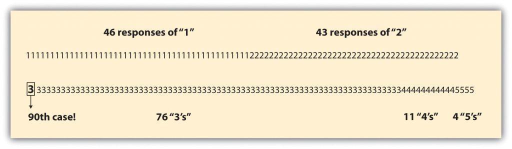
In Figure 12.2, the value of each response to the financial security question is noted, and the middle point within that range of responses is highlighted. To find the middle point, we simply divide the number of valid cases by two. The number of valid cases, 180, divided by 2 is 90, so we’re looking for the 90th value on our distribution to discover the median. As you’ll see in Figure 12.2, that value is 3; thus, the median on our financial security question is 3 or “moderately secure.”
As you can see, we can learn a lot about our respondents simply by conducting univariate analysis of measures on our survey. We can learn even more, of course, when we begin to examine relationships across multiple variables. This latter type of analysis is known as multivariate analysis.
Bivariate analysis allows us to assess covariation among two variables. We reviewed covariation in Chapter 7. This means we can find out whether changes in one variable occur together with changes in another. If two variables do not covary, they are said to have independence, which simply means that there is no relationship between the two variables in question. To learn whether a relationship exists between two variables, a researcher may cross-tabulate the two variables and present their relationship in a contingency table. A contingency table shows how variation on one variable may be contingent on variation on the other.
Let’s look at a contingency table to get a visual representation. In Table 12.4, I have cross-tabulated two questions from an older worker survey: respondents’ reported gender and their self-rated financial security.
| Men | Women | |
| Not financially secure (%) | 44.1 | 51.8 |
| Moderately financially secure (%) | 48.9 | 39.2 |
| Financially secure (%) | 7.0 | 9.0 |
| Total | N = 43 | N = 135 |
In Table 12.4, you’ll notice that I collapsed a few of the financial security response categories (recall there were five categories presented in Table 12.3). Sometimes researchers will collapse response categories on similar items to make the results easier to read. You’ll also see that I placed the variable “gender” in the table’s columns and “financial security” in its rows. Typically, values that are contingent on other values (dependent variables) are placed in rows, while independent variables are placed in columns. This simplifies the comparison across categories of our independent variable.
Reading across the top row of our table, we can see that around 44% of men in the sample reported that they are not financially secure while almost 52% of women reported the same. In other words, more women than men reported they are not financially secure. You’ll also see in the table that I reported the total number of respondents for each category of the independent variable in the table’s bottom row. This is also standard practice in a bivariate table, as is including a table heading describing what is presented in the table.
Researchers interested in simultaneously analyzing relationships among more than two variables conduct multivariate analysis. If I hypothesized that financial security declines for women as they age but increases for men as they age, I might consider adding age to the preceding analysis. To do so would require multivariate, rather than bivariate, analysis. This is common in studies with multiple independent or dependent variables. It is also necessary for studies that include control variables, which almost all studies do. We won’t go into detail about how to conduct multivariate analysis of quantitative survey items here. If you are interested in learning more about the analysis of quantitative survey data, I recommend checking out your campus’s offerings in statistics classes. The quantitative data analysis skills you will gain in a statistics class could serve you quite well should you find yourself seeking employment one day.
Key Takeaways
- While survey researchers should always aim to obtain the highest response rate possible, some recent research argues that high return rates on surveys may be less important than we once thought.
- There are several computer programs designed to assist quantitative researchers with analyzing their data include SPSS, MicroCase, and Excel.
- Data analysis is about identifying, describing, and explaining patterns.
- Contingency tables show how one variable may covary with another.
Glossary
Bivariate analysis– quantitative analysis that examines relationships among two variables
Codebook- a document that outlines how a survey researcher has translated their data from words into numbers
Contingency table- shows how variation on one variable may be contingent on variation on the other
Frequency distribution- summarizes the distribution of responses on a single survey question
Independence- there is no relationship between the two variables in question
Mean- also known as the average, this is the sum of the value of all responses on a given variable divided by the total number of responses
Median- the value that lies in the middle of a distribution of responses
Mode- the most common response given to a question
Multivariate analysis- quantitative analysis that examines relationships among more than two variables
Nonresponse bias- bias-reflected differences between people who respond to your survey and those who do not respond
Response rate- the number of people who respond to your survey divided by the number of people to whom the survey was distributed
Univariate analysis- quantitative analysis that describes patterns across just one variable
- Langer, G. (2003). About response rates: Some unresolved questions. Public Perspective, May/June, 16–18. Retrieved from: https://www.aapor.org/AAPOR_Main/media/MainSiteFiles/Response_Rates_-_Langer.pdf ↵
- Curtin, R., Presser, S., & Singer, E. (2000). The effects of response rate changes on the index of consumer sentiment. Public Opinion Quarterly, 64, 413–428; Keeter, S., Kennedy, C., Dimock, M., Best, J., & Craighill, P. (2006). Gauging the impact of growing nonresponse on estimates from a national RDD telephone survey. Public Opinion Quarterly, 70, 759–779; Merkle, D. M., & Edelman, M. (2002). Nonresponse in exit polls: A comprehensive analysis. In M. Groves, D. A. Dillman, J. L. Eltinge, & R. J. A. Little (Eds.), Survey nonresponse (pp. 243–258). New York, NY: John Wiley and Sons. ↵
- Figure 12.2 copied from Blackstone, A. (2012). Principles of sociological inquiry: Qualitative and quantitative methods. Saylor Foundation. Retrieved from: https://saylordotorg.github.io/text_principles-of-sociological-inquiry-qualitative-and-quantitative-methods/ Shared under CC-BY-NC-SA 3.0 License (https://creativecommons.org/licenses/by-nc-sa/3.0/) ↵
